Introduction:
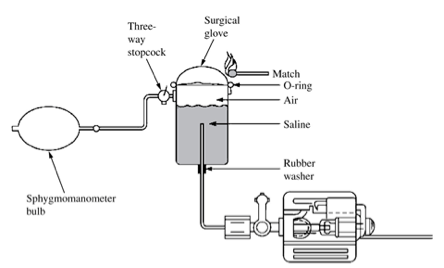
In this exercise, you will measure pressure changes in a fluid-filled container using a fluid-filled pressure transducer. You will gradually increase the pressure inside the container until the rubber glove mounted on the container flies off due to the pressure. The sudden pressure drop will yield a Step Response, which can be measured and characterized using LabView.
 Theory:
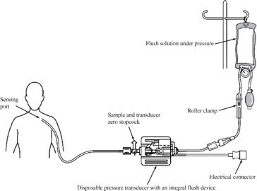
For direct measurements of blood pressure in arteries and veins, fluid-filled pressure transducers are used (e.g. in surgical theaters and intensive care units). This requires direct access to the blood vessel you wish to measure the pressure in. The pressure itself is measured using a transducer, which is located outside the body, but which is connected to the vessel through a fluid-filled tube.
Due to the fluid inertia, the fluid resistance and compliance in the measurement membrane, the catheter system can be modelled as a second order lowpass system:

This second order system will be measured and characterized. We will use a pre-made setup like the one below, which will enable the measurement of the step response of the catheter. However, we will not be using the burning match, as the rubber gloves are to be reused.

Setup:
Materials:
- A plastic cylinder
- Fluid filled transducer
- Amplifier for the transducer
- Rubber glove
- 4 cables with banana-plugs (male-male)
- Cable: Amplifier -> 2 naked wires
- 1 DAQ (NI-6009)
Instructions:
- Insert the long tube in the pressure-transducer and connect the other end to the cylinder, which has an attachment tube at the bottom.
- Turn the three-way connector, so there is connection from the cylinder to the pressure-transducer.
- Fill the cylinder up to 4/5 using water.
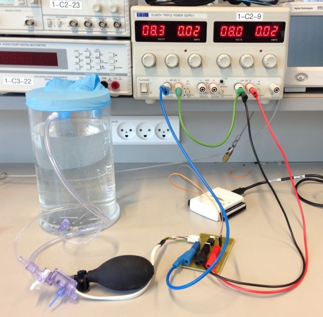
- Hold a paper towel behind the open connection of the transducer and pull on the dark blue rubber until water dribbles out of the open tube (see the top picture). Then let go of the rubber string - this will ensure that the tube is filled with water, and that there are no air bubbles present.
- Turn off the lab power supplies on the little round buttons next to the positive terminals, so that there is light inside the screens, but not in the diodes. Adjust the power supply to +8V on both circuits and adjust the current to 0.02 A. You will need both a positive and a negative voltage, which you will acquire by connecting the left + terminal (red) to the right - terminal (black) and setting both supplies to 8V. Connect Ground to the black input of the amplifier, +8V to the red input and -8V to the blue input (see the image below).
- Verify that everything is connected correctly - please ask the teacher if you have any question at all!
- Connect the pressure-transducer to the amplifier and turn on the power supplies.
- Connect the cable with the two naked wires to your DAQ on input AI0
- Put a glove over the cylinder

VI implementation:
In this exercise, you will create a VI, which can measure the step-respones when the glove flies off the cylinder. The raw signal is saved to the LVM format. Subsequently, a new VI is created, which will load the saved LVM signal, in which functions are used to discard the irrelevant data leaving only the Step Response (Extract Portion of a Signal & Trigger and Gate). The extracted step response signal will then be analyzed using a Peaks/Valley detector, which will detect peaks and valleys on the signal, as well as the overall maximum and minimum.
Data input:
- Start LabView and create an empty VI.
- Insert a DAQ assistant on the Block Diagram
- Acquire Signal -> Analog Input -> Voltage
- Set Acquisition mode (bottom) to Continuous Samples and Samples to Read = 10 and Rate (Hz) = 1000.
- The DAQ has to read the number of samples you set here, before submitting data. If you set it to 1000, it will have to read data for 1 second (Rate = 1000 Hz) before sending the data onwards. This would create a very jagged graph - to smooth the output, the Samples to Read is restricted to 10 - so the signal will be updated every 10/1000 seconds, i.e. 100 times/second.
- Click OK and answers Yes to insert a While Loop
- Connect Data from the DAQ assistant with a Waveform Graph and a numerical indicator.
- Run the VI, and increase the pressure using the rubber ball. Check that the pressure increase is reflected in the curves.
- You will now save the data. Insert a Case structure into the While Loop and connect the Selector terminal to a Boolean Control (Mechanical Action = Switch). Rename the control "Save data".
- Insert a "Write To Measurement File" Express VI in the True case. Save the data as StepResponseData.lvm.
Set Segment Headers to "No Headers" and X Value (Time Columns) to "One column only". Set the function to "Overwrite file" under the heading "If a file already exists". - Wire the Data output from the DAQ assistant to the Signals input of the "Write To Measurement File" Express VI
- Set the status of "Save Data" to True, and run the VI while increasing pressure with the rubber ball, until the glove flies off. A second or two thereafter, you can stop the VI.
- Save your VI as 4.2 - StepResponseInput.vi
Data analysis:
- Create a new empty VI.
- Open your data file "StepResponseData.lvm" in Notepad. Find the last value. As the sampling frequency is 1000 Hz, there will be 1000 times this value of datapoints + 1 (time is zero-indexed). Note this number, and the maximal time value.
- Insert a "Read From Measurement File" and set the filename to the name of the file saved earlier (StepResponseData.lvm)
- Under "Segment Size" you will enter the number of sampled you read in notepad.
- Press OK
- Insert a Waveform Graph and rename it "Input Signal". Disable "Autoscale X" and set the max-value of the X-axis to be the maximal time value, read in Notepad.
- Connect Input Signal with the Signals output from the "Read From Measurement File" Express VI.
- Run your VI and check that the signal is read and plotted correctly.
We now need to crop the signal roughly:
- Insert an "Extract Portion of Signal" Express VI and connect it to the Signal output from "Read From Measurement File"
- Choose "Begin at offset (x-axis units)" (just leave the offset at 0)
- Set Duration or Span to "Remaining samples"
- Press OK
- Insert an "Array Max & Min" function and connect the input with the Signals output from "Read From Measurement File"
- Insert a Division function and connect the top input to the max index(es) from "Array Max & Min". Wire a constant of 1000 to the bottom input
- This value represents the time at which the maximal value of the signal appears. The reason for dividing by 1000, is that the signal is sampled at 1000 Hz, and the function displays the index at which the signal was maximal - not the time. Thus, dividing with 1000 yield the time of the maximal signal.
- Expand "Extract Portion…" maximally downwards.
- Connect "Begin Offset" to the output from the division function and Signals to the signal from the "Read From Measurement File"
- Create a new Waveform Graph and rename it "Cropped Signal". Connect the Section output from the "Extract Portion of Signal" VI to "Cropped Signal"
- Run the VI again and check that the "Cropped Signal" contains the step response.
Now the signal will be finely cropped, so that it only contains the Step Response itself:
- Insert a "Trigger and Gate" Express VI
- Set "Threshold" to "Start sense = Falling" and the "Start level" to the value immediately prior to the Step Response.
- Read on the "Cropped Signal" graph, approximately how long it takes from the beginning of the Step Response until the end. Multiply the time with 1000 (Hz), which will yield the "Number of samples". Enter this value in "Stop Trigger".
- Press OK
- Connect the Signals input to the Section output from the "Extract Portion…" VI
- This signal will now be plotted in an XY-graph
- The reason for choosing this plot-type rather than a Waveform Graph is, that it will allow simultaneous display of the Step Response itself, as well as the peaks and valleys, we will detect below. This will be done by bundling the individual components X- and Y-values and finally, before all three are displayed, by building an Array containing all three bundles.
- To be able to plot the Step Response in an XY-graph, it needs both X and Y coordinates. The latter is already found, as this will be the voltage signal itself. The X-values must be set to a linear increasing function, exactly the length of the number of signals from the "Trigger and Gate" VI:
- First the dynamic data from the "Trigger and Gate" VI will be converted:
- Insert a "Convert from Dynamic Data" function and connect it to the "Triggered Signal" output from the "Trigger and Gate" function.
- Insert a "Bundle Data" function and connect the bottom input to the output from "Convert from Dynamic Data"
- The top input will consist of a 1D-array containing the numbers 1 to the number of samples:
- Insert a "Ramp Pattern" function and an "Array Size" function
- Connect the "Array Size" function to the "Convert From Dynamic Data" function.
- The output from "Array Size" is connected to the "Samples" input on the "Ramp Pattern" function
- Insert a decrement ("-1") function from Programming->Numeric and connect it to the output from "Convert From Dynamic Data" and the input "end" on the "Ramp Pattern" function
- Connect the output from "Ramp Pattern" to the top input of "Bundle Data"
- Insert an XY-graph on the Front Panel and rename it "Step Response".
- Connect the output from the "Bundle Data" function to a "Build Array" function (leave it 1 long).
- Connect the Build Array function to the XY-graph "Step Response"
- Run your VI and check that the "Step Response" graph actually shows the Step Response.
- First the dynamic data from the "Trigger and Gate" VI will be converted:
Finally the Step Response will be analyzed, max and min values found and Peaks/Valleys marked
- Insert a "Transition Measurements" VI and connect the Section output from the "Extract Portion" VI to the input to the top left. Set "polarity" to "falling" and connect slope, transition duration, and the post-transition exits with indicators.
- Insert an "Array Max & Min" function and connect it to the exit from "Convert from Dynamic Data". Create an indicator of both max and min values.
- Insert a Peak Detector function and connect the X input to the output from "Convert from Dynamic Data"
- Create a constant on the peaks/valleys input to the bottom left and choose "Peaks"
- Create a "Bundle" function and connect the "Locations" output from the "Peak Detector" to the top input and Amplitudes to the bottom. Expand the "Build Array" function to be 2 rows and connect the exit from the bundle function to another input to the "Build Array" function.
- Run your VI and check, that Peaks are now marked.
- If your signal is noisy, you will have too many peaks.
- In that case, insert a low-pass filter on the Signals output from the "Read from Measurement File" VI and choose e.g. a cutoff frequency of 50 Hz (Express -> Signal Analysis -> Filter).
- Connect the output with the Signals input of "Extract Portion of Signal"
- Change the plot type for the peaks by expanding the legend and left-clicking the second plot and choosing "Common Plots" -> dots
- Copy the "Peak Detector" function and create a constant on the peaks/valleys input to the bottom left and choose "Valleys"
- However, these will not be detected until the Thrshold is set to a value higher than the measured (the default is 0). Therefore, connect the "Threshold" input to the max-value from the "Array Max & Min" function.
- Create a bundle, wire as before and expand the "Build Array" funtion to 3 rows - connect the bottom one with the output from the "Valley" bundle.
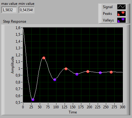
- Run your VI and check, that the Step Response graph looks approximately like below
- (Right-click the graph and choos "Properties" to adjust colors, symbols, grid line color etc.)
- Save your VI as "4.2 - StepResponseAnalysis.vi"
